

Binary classification on PIMA Indian Dataset
This problem is comprised of 768 observations of medical details for Pima indians patents. The records describe instantaneous measurements taken from the patient such as their age, the number of times pregnant and blood workup. All patients are women aged 21 or older. All attributes are numeric, and their units vary from attribute to attribute.
Each record has a class value that indicates whether the patient suffered an onset of diabetes within 5 years of when the measurements were taken (1) or not (0).
The goal is to predict whether or not a given female patient will contract diabetes based on features such as BMI, age, and number of pregnancies. Therefore, it is a binary classification problem. A target value of 0 indicates that the patient does not have diabetes, while a value of 1 indicates that the patient does have diabetes.
There may be some missing values with which you have to deal with.
Build a prediction Algorithm using Decision Tree.
import numpy as np
import pandas as pd
import seaborn as sns
import matplotlib.pyplot as plt
from sklearn.model_selection import train_test_split
from sklearn.preprocessing import StandardScaler
from sklearn.tree import DecisionTreeClassifier,plot_tree
from sklearn.metrics import mean_absolute_error, accuracy_score, confusion_matrix
df=pd.read_csv(r"D:\Learning\DLithe-ML\Assignment\diabetes.csv")
df.shape
(768, 9)
df.info()
<class 'pandas.core.frame.DataFrame'>
RangeIndex: 768 entries, 0 to 767
Data columns (total 9 columns):
 #   Column                    Non-Null Count  Dtype
---  ------                    --------------  -----
 0   Pregnancies               768 non-null    int64
 1   Glucose                   768 non-null    int64
 2   BloodPressure             768 non-null    int64
 3   SkinThickness             768 non-null    int64
 4   Insulin                   768 non-null    int64
 5   BMI                       768 non-null    float64
 6   DiabetesPedigreeFunction  768 non-null    float64
 7   Age                       768 non-null    int64
 8   Outcome                   768 non-null    int64
dtypes: float64(2), int64(7)
memory usage: 54.1 KB
df=df.drop_duplicates()
df.shape
(768, 9)
df.isnull().sum()
Pregnancies                 0
Glucose                     0
BloodPressure               0
SkinThickness               0
Insulin                     0
BMI                         0
DiabetesPedigreeFunction    0
Age                         0
Outcome                     0
dtype: int64
df.head().T
| 0 | 1 | 2 | 3 | 4 | |
|---|---|---|---|---|---|
| Pregnancies | 6.000 | 1.000 | 8.000 | 1.000 | 0.000 |
| Glucose | 148.000 | 85.000 | 183.000 | 89.000 | 137.000 |
| BloodPressure | 72.000 | 66.000 | 64.000 | 66.000 | 40.000 |
| SkinThickness | 35.000 | 29.000 | 0.000 | 23.000 | 35.000 |
| Insulin | 0.000 | 0.000 | 0.000 | 94.000 | 168.000 |
| BMI | 33.600 | 26.600 | 23.300 | 28.100 | 43.100 |
| DiabetesPedigreeFunction | 0.627 | 0.351 | 0.672 | 0.167 | 2.288 |
| Age | 50.000 | 31.000 | 32.000 | 21.000 | 33.000 |
| Outcome | 1.000 | 0.000 | 1.000 | 0.000 | 1.000 |
# Print number of missing values by count
print((df[['Glucose', 'BloodPressure', 'SkinThickness', 'Insulin', 'BMI', 'DiabetesPedigreeFunction', 'Age']] == 0).sum())
Glucose                       5
BloodPressure                35
SkinThickness               227
Insulin                     374
BMI                          11
DiabetesPedigreeFunction      0
Age                           0
dtype: int64
# Replace all 0 with NaN
df[['Glucose', 'BloodPressure', 'SkinThickness', 'Insulin', 'BMI']] = df[['Glucose', 'BloodPressure', 'SkinThickness', 'Insulin', 'BMI']].replace(0, np.NaN)
# print the first 5 rows of data
df.head().T
| 0 | 1 | 2 | 3 | 4 | |
|---|---|---|---|---|---|
| Pregnancies | 6.000 | 1.000 | 8.000 | 1.000 | 0.000 |
| Glucose | 148.000 | 85.000 | 183.000 | 89.000 | 137.000 |
| BloodPressure | 72.000 | 66.000 | 64.000 | 66.000 | 40.000 |
| SkinThickness | 35.000 | 29.000 | NaN | 23.000 | 35.000 |
| Insulin | NaN | NaN | NaN | 94.000 | 168.000 |
| BMI | 33.600 | 26.600 | 23.300 | 28.100 | 43.100 |
| DiabetesPedigreeFunction | 0.627 | 0.351 | 0.672 | 0.167 | 2.288 |
| Age | 50.000 | 31.000 | 32.000 | 21.000 | 33.000 |
| Outcome | 1.000 | 0.000 | 1.000 | 0.000 | 1.000 |
# count the number of NaN (null) values in each column
print(df.isnull().sum())
Pregnancies                   0
Glucose                       5
BloodPressure                35
SkinThickness               227
Insulin                     374
BMI                          11
DiabetesPedigreeFunction      0
Age                           0
Outcome                       0
dtype: int64
# Replace the null values with the mean of that column
df = df.fillna(df.mean())

# Check the number of null values after replacing
print(df.isnull().sum())
Pregnancies                 0
Glucose                     0
BloodPressure               0
SkinThickness               0
Insulin                     0
BMI                         0
DiabetesPedigreeFunction    0
Age                         0
Outcome                     0
dtype: int64
df.head().T
| 0 | 1 | 2 | 3 | 4 | |
|---|---|---|---|---|---|
| Pregnancies | 6.000000 | 1.000000 | 8.000000 | 1.000 | 0.000 |
| Glucose | 148.000000 | 85.000000 | 183.000000 | 89.000 | 137.000 |
| BloodPressure | 72.000000 | 66.000000 | 64.000000 | 66.000 | 40.000 |
| SkinThickness | 35.000000 | 29.000000 | 29.153420 | 23.000 | 35.000 |
| Insulin | 155.548223 | 155.548223 | 155.548223 | 94.000 | 168.000 |
| BMI | 33.600000 | 26.600000 | 23.300000 | 28.100 | 43.100 |
| DiabetesPedigreeFunction | 0.627000 | 0.351000 | 0.672000 | 0.167 | 2.288 |
| Age | 50.000000 | 31.000000 | 32.000000 | 21.000 | 33.000 |
| Outcome | 1.000000 | 0.000000 | 1.000000 | 0.000 | 1.000 |
df.columns
Index(['Pregnancies', 'Glucose', 'BloodPressure', 'SkinThickness', 'Insulin',
       'BMI', 'DiabetesPedigreeFunction', 'Age', 'Outcome'],
      dtype='object')
a = ['Pregnancies', 'Glucose', 'BloodPressure', 'SkinThickness', 'Insulin','BMI', 'DiabetesPedigreeFunction', 'Age']
b = ['Outcome']
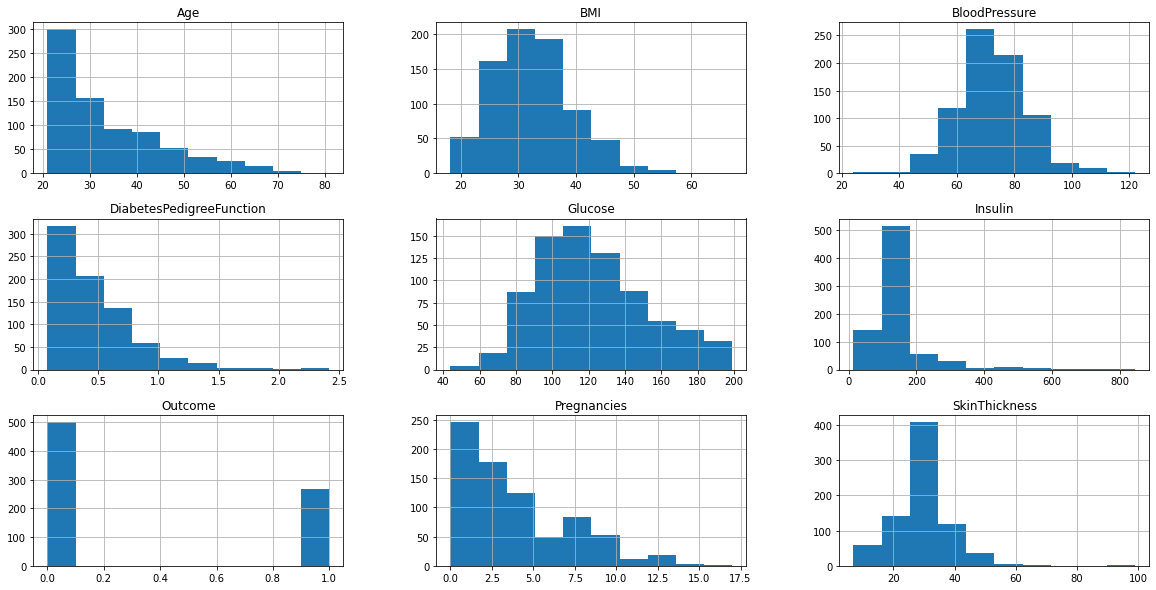
plt.rcParams['figure.figsize'] = (20, 10)
df.hist()
plt.show()
plt.rcParams['figure.figsize'] = (6, 5)
sns.countplot(x="Outcome",data=df)
plt.show()
print(df["Outcome"].value_counts())

0    500
1    268
Name: Outcome, dtype: int64
This shows that there are 500 negative results and 268 positive results
for i in a:
    sns.swarmplot(x="Outcome",y=i,data=df)
    plt.show()
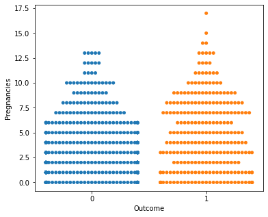
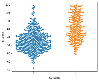
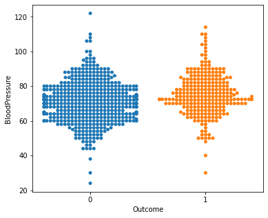
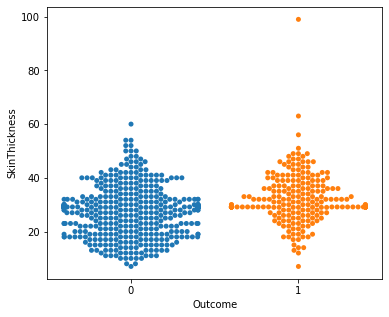
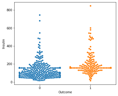
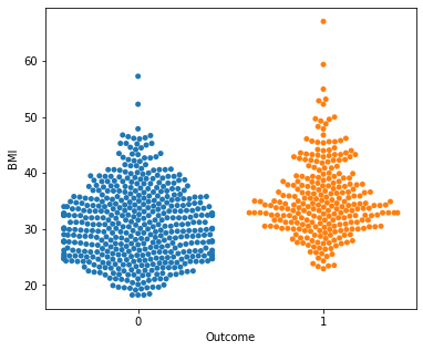
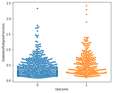
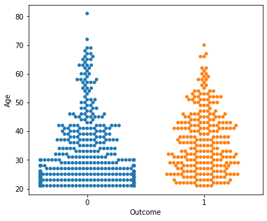
No clear conclusions can be drawn from the above swarmplots
But these are some readings that could prove useful:
Women with more than 13 pregnancies tend to get diabetes
Women with glucose less than 75 tend to NOT get diabetes.
for i in a:
    print(df[i].describe())
    print(df[i].skew())
    sns.distplot(df[i], kde=False)
    plt.show()
count    768.000000
mean       3.845052
std        3.369578
min        0.000000
25%        1.000000
50%        3.000000
75%        6.000000
max       17.000000
Name: Pregnancies, dtype: float64
0.9016739791518588
count    768.000000
mean     121.686763
std       30.435949
min       44.000000
25%       99.750000
50%      117.000000
75%      140.250000
max      199.000000
Name: Glucose, dtype: float64
0.5327186599872982
count    768.000000
mean      72.405184
std       12.096346
min       24.000000
25%       64.000000
50%       72.202592
75%       80.000000
max      122.000000
Name: BloodPressure, dtype: float64
0.13730536744146796
count    768.000000
mean      29.153420
std        8.790942
min        7.000000
25%       25.000000
50%       29.153420
75%       32.000000
max       99.000000
Name: SkinThickness, dtype: float64
0.8221731383793047
count    768.000000
mean     155.548223
std       85.021108
min       14.000000
25%      121.500000
50%      155.548223
75%      155.548223
max      846.000000
Name: Insulin, dtype: float64
3.019083661355125
count    768.000000
mean      32.457464
std        6.875151
min       18.200000
25%       27.500000
50%       32.400000
75%       36.600000
max       67.100000
Name: BMI, dtype: float64
0.5982526551146302
count    768.000000
mean       0.471876
std        0.331329
min        0.078000
25%        0.243750
50%        0.372500
75%        0.626250
max        2.420000
Name: DiabetesPedigreeFunction, dtype: float64
1.919911066307204
count    768.000000
mean      33.240885
std       11.760232
min       21.000000
25%       24.000000
50%       29.000000
75%       41.000000
max       81.000000
Name: Age, dtype: float64
1.1295967011444805
From the above distplots, we can make the following conclusions:
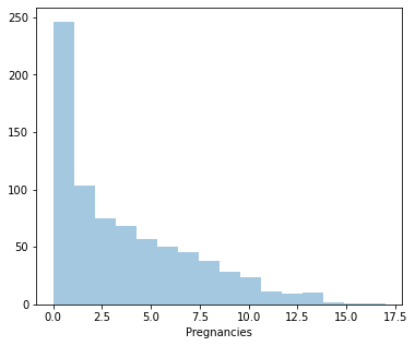
Distplot 1 : Pregnancies
Least Pregnancy: 0
Highest Pregnancy: 17
Average Pregnancy: 4
Since it’s positively skewed - Majority of the women have fewer pregnancies.
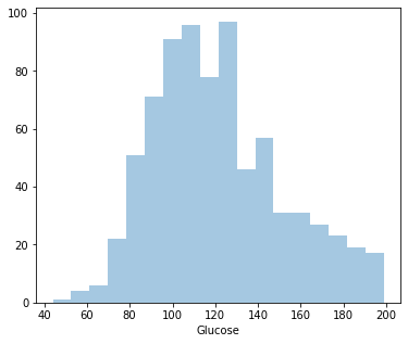
Distplot 2 : Glucose
Least Glucose level: 44
Highest Glucose level: 199
Average Glucose level: 121.68
Since it’s positively skewed - Majority of the women have lower glucose level.
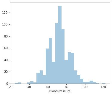
Distplot 3 : Blood Pressure
Least Blood Pressure: 24 mm Hg
Highest Blood Pressure: 122 mm Hg
Average Blood Pressure: 72.40 mm Hg
Since it’s positively skewed - Majority of the women have a lower Blood Pressure.
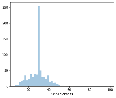
Distplot 4 : Skin Thickness
Least Skin Thickness: 7 mm
Highest Skin Thickness: 99 mm
Average Skin Thickness: 29.15 mm
Since it’s positively skewed - Majority of the women have a lower Skin Thickness.
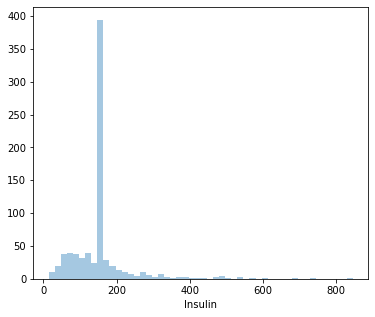
Distplot 5 : Insulin
Least Insulin level: 14 U/ml
Highest Insulin level: 846 U/ml
Average Insulin level: 155.54 U/ml
Since it’s positively skewed - Majority of the women have a lower insulin level.
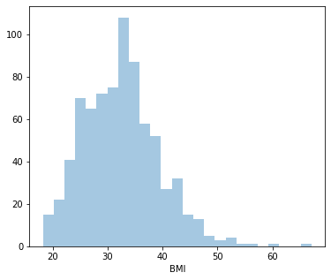
Distplot 6 : BMI
Least BMI: 18.20
Highest BMI: 67.10
Average BMI: 32.45
Since it’s positively skewed - Majority of the women have a lower BMI.
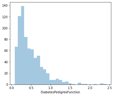
Distplot 7 : DiabetesPedigreeFunction
Least value: 0.078
Highest value: 2.420
Average value: 0.471
Since it’s positively skewed - Majority of the women have a lower DiabetesPedigreeFunction value.
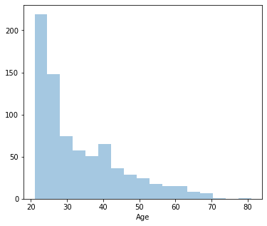
Distplot 8 : Age
Least age: 21
Highest age: 33
Average age: 81
Since it’s positively skewed - Majority of the women are younger.
print(df.skew())
Pregnancies                 0.901674
Glucose                     0.532719
BloodPressure               0.137305
SkinThickness               0.822173
Insulin                     3.019084
BMI                         0.598253
DiabetesPedigreeFunction    1.919911
Age                         1.129597
Outcome                     0.635017
dtype: float64
Insulin and DiabetesPedigreeFunction are highly skewed data. So we will normalize by using the log values of the colulmns
df['Insulin'] = np.log(df['Insulin'])
print("skew: ", df['Insulin'].skew())
sns.distplot(df['Insulin'], kde=False)
plt.show()
print('-'*40)
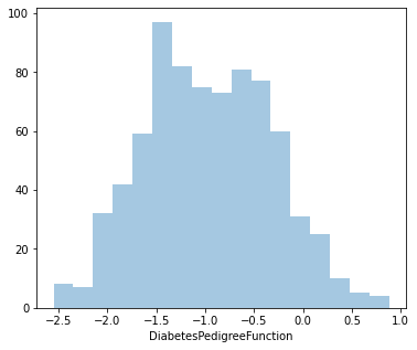
df['DiabetesPedigreeFunction'] = np.log(df['DiabetesPedigreeFunction'])
print("skew: ", df['DiabetesPedigreeFunction'].skew())
sns.distplot(df['DiabetesPedigreeFunction'], kde=False)
plt.show()
skew: -0.7896950416949489
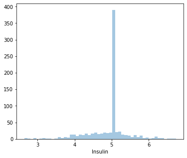
----------------------------------------
skew:  0.11417768826564408
Machine Learning model - Decision Tree
# Split the dependent and independent values
x = df.drop("Outcome",axis=1)
y = df["Outcome"]
# pre-processing the data
x = StandardScaler().fit(x).transform(x)
# Split the data for training and testing
xtrain, xtest, ytrain, ytest = train_test_split(x, y, train_size=0.7)
print ('Train set:', xtrain.shape,  ytrain.shape)
print ('Test set:', xtest.shape,  ytest.shape)
Train set: (537, 8) (537,)
Test set: (231, 8) (231,)
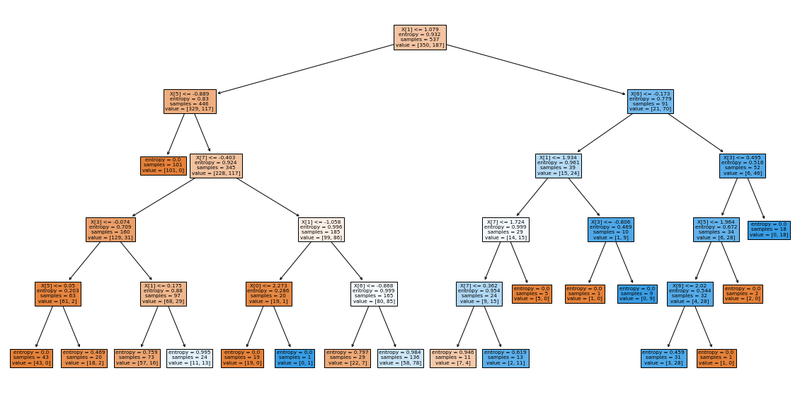
# Load decision tree classifier model from sklearn and fit the training sets
algo = DecisionTreeClassifier(criterion='entropy',max_depth=5)
algo.fit(xtrain,ytrain)
DecisionTreeClassifier(criterion='entropy', max_depth=5)
plt.figure(figsize=(20,10))
plot_tree(algo,filled=True)
plt.show()
ypred = algo.predict(xtest)

# compare predicted values and actual values and find out accuracy
print("Accuracy: ", accuracy_score(ytest,ypred))
Accuracy: 0.7445887445887446
print(confusion_matrix(ytest,ypred))
[[112  38]
 [ 21  60]]