Model to predict power output of a peaker power plant

The dataset contains 9568 data points collected from a Combined Cycle Power Plant over 6 years (2006-2011), when the power plant was set to work with full load. Features consist of hourly average ambient variables Temperature (T), Ambient Pressure (AP), Relative Humidity (RH) and Exhaust Vacuum (V) to predict the net hourly electrical energy output (EP) of the plant.

The power output of a peaker power plant varies depending on environmental conditions, so the business problem is predicting the power output of a peaker power plant as a function of the environmental conditions – since this would enable the grid operator to make economic tradeoffs about the number of peaker plants to turn on (or whether to buy expensive power from another grid).

import numpy as np
import pandas as pd
import seaborn as sns
import matplotlib.pyplot as plt
from sklearn.model_selection import train_test_split
from sklearn.linear_model import LinearRegression
from sklearn.metrics import mean_absolute_error, r2_score
from sklearn.preprocessing import StandardScaler

df=pd.read_csv(r"D:\Learning\DLithe-ML\Assignment\combined_cycle_power_plant.csv", sep=";")

df.shape

(9568, 5)

df.info()

<class 'pandas.core.frame.DataFrame'>
RangeIndex: 9568 entries, 0 to 9567
Data columns (total 5 columns):
 #   Column             Non-Null Count  Dtype  
---  ------             --------------  -----  
 0   temperature        9568 non-null   float64
 1   exhaust_vacuum     9568 non-null   float64
 2   ambient_pressure   9568 non-null   float64
 3   relative_humidity  9568 non-null   float64
 4   energy_output      9568 non-null   float64
dtypes: float64(5)
memory usage: 373.9 KB

df=df.drop_duplicates()
df.shape

(9527, 5)

df.isnull().sum()

temperature          0
exhaust_vacuum       0
ambient_pressure     0
relative_humidity    0
energy_output        0
dtype: int64

df.head().T

	0	1	2	3	4
temperature	9.59	12.04	13.87	13.72	15.14
exhaust_vacuum	38.56	42.34	45.08	54.30	49.64
ambient_pressure	1017.01	1019.72	1024.42	1017.89	1023.78
relative_humidity	60.10	94.67	81.69	79.08	75.00
energy_output	481.30	465.36	465.48	467.05	463.58

a=["temperature", "exhaust_vacuum", "ambient_pressure", "relative_humidity", "energy_output"]

for i in a:
    print(df[i].describe())
    print(df[i].skew())
    sns.distplot(df[i], kde=False)
    plt.show()

count    9527.000000
mean       19.658225
std         7.444397
min         1.810000
25%        13.530000
50%        20.350000
75%        25.710000
max        37.110000
Name: temperature, dtype: float64
-0.1361069178515444

count    9527.000000
mean       54.293421
std        12.686309
min        25.360000
25%        41.740000
50%        52.080000
75%        66.510000
max        81.560000
Name: exhaust_vacuum, dtype: float64
0.1968187812768364

count    9527.000000
mean     1013.237084
std         5.940526
min       992.890000
25%      1009.085000
50%      1012.920000
75%      1017.200000
max      1033.300000
Name: ambient_pressure, dtype: float64
0.273845628693525

count    9527.000000
mean       73.334951
std        14.607513
min        25.560000
25%        63.375000
50%        75.000000
75%        84.850000
max       100.160000
Name: relative_humidity, dtype: float64
-0.43513848893895307

count    9527.00000
mean      454.33591
std        17.03908
min       420.26000
25%       439.75000
50%       451.52000
75%       468.36500
max       495.76000
Name: energy_output, dtype: float64
0.3057905126118896

From the above distplots, we can make the following conclusions:
(All the ambient variables are taken on an hourly average basis.)

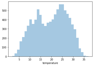
Distplot 1 : Temperature

Least Temperature: 1.81°C
Highest Temperature: 37.11°C
Average Temperature: 19.65°C

Since it’s negatively skewed - Majority of the power plants have a higher temperature

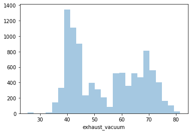
Distplot 2 : Exhaust Vacuum

Least Exhaust Vacuum: 25.36 cm Hg
Highest Exhaust Vacuum: 81.56 cm Hg
Average Exhaust Vacuum: 54.29 cm Hg

Since it’s positively skewed - Majority of the power plants have a lower Exhaust Vacuum

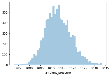
Distplot 3 : Ambient Pressure

Least Ambient Pressure: 992.89 milibar
Highest Ambient Pressure: 1033.30 milibar
Average Ambient Pressure: 1013.23g milibar

Since it’s positively skewed - Majority of the power plants have a lower Ambient Pressure

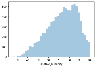
Distplot 4 : Relative Humidity

Least Exhaust Vacuum: 25.56%
Highest Exhaust Vacuum: 100.16%
Average Exhaust Vacuum: 73.33%

Since it’s negatively skewed - Majority of the power plants have a higher Relative Humidity

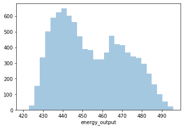
Distplot 5 : Energy Output

Least Energy Output: 420.26 MW
Highest Energy Output: 495.76 MW
Average Energy Output: 454.33 MW

Since it’s negatively skewed - Majority of the power plants have a higher Relative Humidity

sns.pairplot(df)
plt.show()

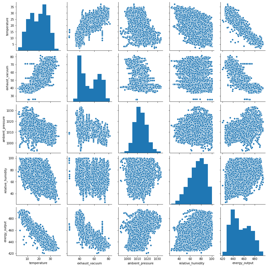
As we can clearly see from the pairplot of Temperature vs Energy Output (or vice-versa) that there is a negative correlation present.

sns.relplot(x="energy_output", y="temperature", data=df)
plt.title('Energy Output vs Temperature', fontsize=20)
plt.show()

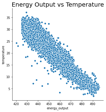
We can safely assume that:
As temperature increases, Energy Output decreases.

Machine Learning model - Linear Regression

# Split the dependent and independent values
x = df.drop("energy_output", axis=1)
y = df["energy_output"]

# pre-processing the data
x = StandardScaler().fit(x).transform(x)

# Split the data for training and testing
xtrain, xtest, ytrain, ytest = train_test_split(x, y, train_size=0.7)

print ('Train set:', xtrain.shape,  ytrain.shape)
print ('Test set:', xtest.shape,  ytest.shape)

Train set: (6668, 4) (6668,)
Test set: (2859, 4) (2859,)

# Load linear regression model from sklearn and fit the training sets
algo=LinearRegression().fit(xtrain, ytrain)

# find out the predictions for the testing set
ypred = algo.predict(xtest)

# compare predicted values and actual values and find out accuracy

print("Mean Absolute Error: ", mean_absolute_error(ytest,ypred))
print("Accuracy: ", r2_score(ytest,ypred))

Mean Absolute Error:  3.602932416142143
Accuracy:  0.9306277586738139