Binary classification on Titanic Dataset

This is a classic dataset used in many data mining tutorials and demos – perfect for getting started with exploratory analysis and building binary classification models to predict survival.

Data covers passengers only, not crew.

import numpy as np
import pandas as pd
import seaborn as sns
import matplotlib.pyplot as plt
from sklearn.preprocessing import LabelEncoder
from sklearn.model_selection import train_test_split
from sklearn.linear_model import LogisticRegression
from sklearn.metrics import mean_absolute_error, accuracy_score
from sklearn.preprocessing import StandardScaler

df=pd.read_csv(r"D:\Learning\DLithe-ML\Assignment\titanic.csv")

df.shape

(891, 15)

df.info()

<class 'pandas.core.frame.DataFrame'>
RangeIndex: 891 entries, 0 to 890
Data columns (total 15 columns):
 #   Column       Non-Null Count  Dtype  
---  ------       --------------  -----  
 0   survived     891 non-null    int64  
 1   pclass       891 non-null    int64  
 2   sex          891 non-null    object 
 3   age          714 non-null    float64
 4   sibsp        891 non-null    int64  
 5   parch        891 non-null    int64  
 6   fare         891 non-null    float64
 7   embarked     889 non-null    object 
 8   class        891 non-null    object 
 9   who          891 non-null    object 
 10  adult_male   891 non-null    bool   
 11  deck         203 non-null    object 
 12  embark_town  889 non-null    object 
 13  alive        891 non-null    object 
 14  alone        891 non-null    bool   
dtypes: bool(2), float64(2), int64(4), object(7)
memory usage: 92.4+ KB

Data cleaning

# Drop duplicate values

df=df.drop_duplicates()
df.shape

(784, 15)

df.isnull().sum()

survived         0
pclass           0
sex              0
age            106
sibsp            0
parch            0
fare             0
embarked         2
class            0
who              0
adult_male       0
deck           582
embark_town      2
alive            0
alone            0
dtype: int64

‘deck’ is mostly empty so we will drop it in the next step.

Age has 106 null values
embarked and embark_town has 2 null values

# Drop columns which are not needed for our analysis or which are duplicates (another column with values meaning the same)

df=df.drop(["deck", "embarked", "adult_male", "alive", "class"], axis=1)

‘deck’ consists of crew data which is excluded in this dataset.

‘embarked’ consists of abbreviated values of ‘embark_town’

‘adult_male’ can be analysed from ‘who’ column; since only a man has adult_male value as 1

‘alive’ is a duplicate of ‘survived’

‘class’ is the textual representation of ‘pclass’

df.head(10)

	survived	pclass	sex	age	sibsp	parch	fare	who	embark_town	alone
0	0	3	male	22.0	1	0	7.2500	man	Southampton	False
1	1	1	female	38.0	1	0	71.2833	woman	Cherbourg	False
2	1	3	female	26.0	0	0	7.9250	woman	Southampton	True
3	1	1	female	35.0	1	0	53.1000	woman	Southampton	False
4	0	3	male	35.0	0	0	8.0500	man	Southampton	True
5	0	3	male	NaN	0	0	8.4583	man	Queenstown	True
6	0	1	male	54.0	0	0	51.8625	man	Southampton	True
7	0	3	male	2.0	3	1	21.0750	child	Southampton	False
8	1	3	female	27.0	0	2	11.1333	woman	Southampton	False
9	1	2	female	14.0	1	0	30.0708	child	Cherbourg	False

df["age"].describe()

count    678.000000
mean      29.869351
std       14.759076
min        0.420000
25%       20.000000
50%       28.250000
75%       39.000000
max       80.000000
Name: age, dtype: float64

# Fill the empty values in 'age' column to the mean value of age

print('Replacing null values with mean value : ', int(df["age"].mean()))
df["age"] = df["age"].fillna(int(df["age"].mean()))
df.head(10)

Replacing null values with mean value :  29

	survived	pclass	sex	age	sibsp	parch	fare	who	embark_town	alone
0	0	3	male	22.0	1	0	7.2500	man	Southampton	False
1	1	1	female	38.0	1	0	71.2833	woman	Cherbourg	False
2	1	3	female	26.0	0	0	7.9250	woman	Southampton	True
3	1	1	female	35.0	1	0	53.1000	woman	Southampton	False
4	0	3	male	35.0	0	0	8.0500	man	Southampton	True
5	0	3	male	29.0	0	0	8.4583	man	Queenstown	True
6	0	1	male	54.0	0	0	51.8625	man	Southampton	True
7	0	3	male	2.0	3	1	21.0750	child	Southampton	False
8	1	3	female	27.0	0	2	11.1333	woman	Southampton	False
9	1	2	female	14.0	1	0	30.0708	child	Cherbourg	False

# Drop rows with empty (null) values

df=df.dropna()

Exploring the Data

a = ['survived', 'pclass', 'sex','sibsp', 'parch', 'who', 'embark_town', 'alone']
b = ['age', 'fare']

for i in a:
    sns.countplot(x=i, data=df)
    plt.show()
    print(df[i].value_counts())

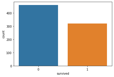
0    461
1    321
Name: survived, dtype: int64

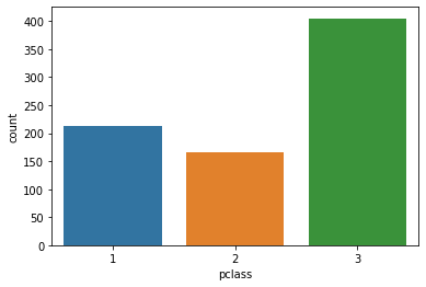
3    405
1    212
2    165
Name: pclass, dtype: int64

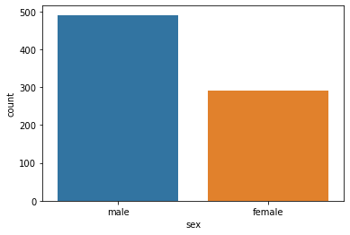
male      491
female    291
Name: sex, dtype: int64

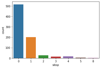
0    515
1    201
2     27
4     18
3     14
5      5
8      2
Name: sibsp, dtype: int64

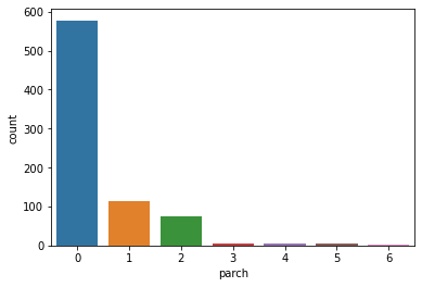
0    578
1    114
2     75
5      5
3      5
4      4
6      1
Name: parch, dtype: int64

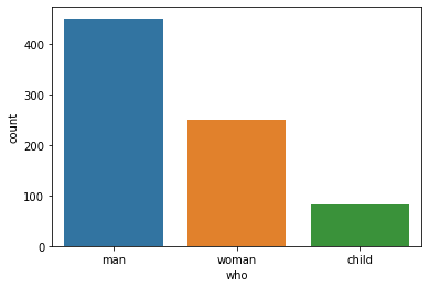
man      451
woman    249
child     82
Name: who, dtype: int64

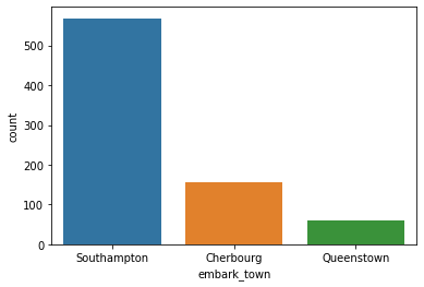
Southampton    568
Cherbourg      155
Queenstown      59
Name: embark_town, dtype: int64

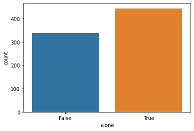
True     444
False    338
Name: alone, dtype: int64

From the above countplots, we can make the following conclusions:

Survived

461 passengers survived while 321 didnt.

Passenger Class

Majority of the passengers were in 3rd class, followed by 1st class and then 2nd class

Sex

Number of male passengers was more than female

Port of Embarkation

Majority of the passengers embarked from Southampton, followed by Cherbourg and the Queenstown

Accompanied

There were more passengers who travelled alone than with others

for i in b:
    print(df[i].describe())
    print(df[i].skew())
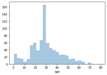
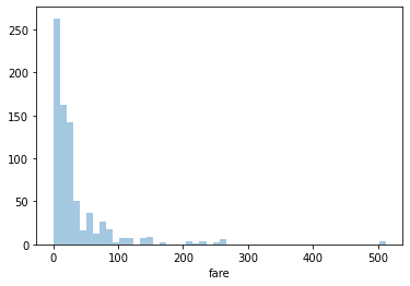
    sns.distplot(df[i], kde=False)
    plt.show()

count    782.000000
mean      29.700026
std       13.692729
min        0.420000
25%       22.000000
50%       29.000000
75%       36.000000
max       80.000000
Name: age, dtype: float64
0.4190340853087404

count    782.000000
mean      34.595913
std       52.176458
min        0.000000
25%        8.050000
50%       15.875000
75%       33.375000
max      512.329200
Name: fare, dtype: float64
4.583205969233933

From the above countplots, we can make the following conclusions:

Age

Youngest: 0.42 (5 months)
Average age: 29
Oldest: 80

Fare

Lowest: 0 (free)
Average: 34.5
Highest: 512

The highly positive skewed data (and the info shown above) proves that 75% of the passengers paid a fare lesser than 34.

sns.swarmplot(x="survived", y="fare", data=df)
plt.show()

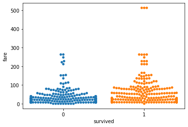
From the figure, we can come to a conclusion that there were a few set of ‘elite’ passengers who paid a very high fare, and were able to survive.

df[['pclass', 'survived']].groupby(['pclass'], as_index=False).mean()

	pclass	survived
0	1	0.627358
1	2	0.509091
2	3	0.256790

sns.countplot(x='pclass',hue="survived", data=df)
plt.show()

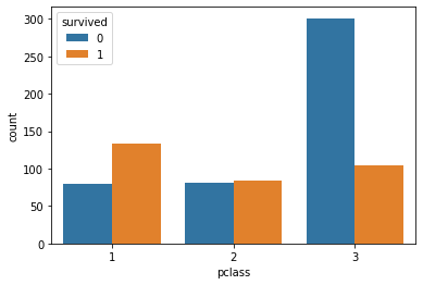
Survival rate was highest in 1st (upper) class and lowest in 3rd class.

Highest number of passengers who survived were from 1st class.

Highest number of passengers who DID NOT survive were from 3rd class.

df[['sex', 'survived']].groupby(['sex'], as_index=False).mean()

	sex	survived
0	female	0.738832
1	male	0.215886

sns.countplot(x='sex',hue="survived", data=df)
plt.show()

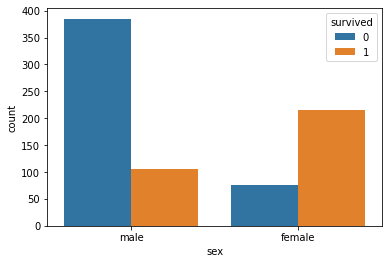
Survival rate of female passengers was more than male

age_survived = sns.FacetGrid(df, col='survived')
age_survived.map(plt.hist, 'age', bins=15)
plt.show()

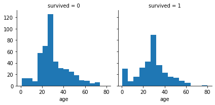
Older passengers (of around 80 years old) survived.

Machine Learning Model - Logistic Regression

# Convert Boolean to Integer

df["alone"] = df["alone"].astype(int)
df.head()

	survived	pclass	sex	age	sibsp	parch	fare	who	embark_town	alone
0	0	3	male	22.0	1	0	7.2500	man	Southampton	0
1	1	1	female	38.0	1	0	71.2833	woman	Cherbourg	0
2	1	3	female	26.0	0	0	7.9250	woman	Southampton	1
3	1	1	female	35.0	1	0	53.1000	woman	Southampton	0
4	0	3	male	35.0	0	0	8.0500	man	Southampton	1

# Encode the data (convert strings to numbers) so that the model can understand.

le_sex = LabelEncoder()
df["sex"]=le_sex.fit_transform(df["sex"])

le_who = LabelEncoder()
df["who"]=le_who.fit_transform(df["who"])

le_embark_town = LabelEncoder()
df["embark_town"]=le_embark_town.fit_transform(df["embark_town"])

print(df.shape)
df.head(10)

(782, 10)

	survived	pclass	sex	age	sibsp	parch	fare	who	embark_town	alone
0	0	3	1	22.0	1	0	7.2500	1	2	0
1	1	1	0	38.0	1	0	71.2833	2	0	0
2	1	3	0	26.0	0	0	7.9250	2	2	1
3	1	1	0	35.0	1	0	53.1000	2	2	0
4	0	3	1	35.0	0	0	8.0500	1	2	1
5	0	3	1	29.0	0	0	8.4583	1	1	1
6	0	1	1	54.0	0	0	51.8625	1	2	1
7	0	3	1	2.0	3	1	21.0750	0	2	0
8	1	3	0	27.0	0	2	11.1333	2	2	0
9	1	2	0	14.0	1	0	30.0708	0	0	0

# Split the dependent and independent values
x = df.drop("survived", axis=1)
y = df["survived"]

# pre-processing the data
x = StandardScaler().fit(x).transform(x)

# Split the data for training and testing
xtrain, xtest, ytrain, ytest = train_test_split(x, y, train_size=0.8)

print ('Train set:', xtrain.shape,  ytrain.shape)
print ('Test set:', xtest.shape,  ytest.shape)

Train set: (625, 9) (625,)
Test set: (157, 9) (157,)

# Load logistic regression model from sklearn and fit the training sets
algo = LogisticRegression().fit(xtrain,ytrain)

# find out the predictions for the testing set
ypred = algo.predict(xtest)

# compare predicted values and actual values and find out accuracy

print("Mean Absolute Error: ", mean_absolute_error(ytest,ypred))
print("Accuracy: ", accuracy_score(ytest,ypred))

Mean Absolute Error:  0.17834394904458598
Accuracy:  0.821656050955414

Highest Accuracy : 0.821656050955414